Introduction to BIRDS
Alejandro Ruete and Debora Arlt
2021-07-21
Source:vignettes/BIRDS.Rmd
BIRDS.RmdInstalling ‘BIRDS’
The package ‘BIRDS’ is currently available on GitHub and you can freely download the source code here BIRDS on GitHub
The easiest option is to install the package directly from GitHub using the package ‘remotes’. Install ’remotes as usual install.packages('remotes') if you do not already have installed it.
remotes::install_github('Greensway/BIRDS')If you receive an error we would love to receive your bug report here
Basic example and data requirements
Starting with a primary biodiversity data set (species observations) BIRDS employs three basic steps: organizing the data into a sampling event-based format, summarizing the data producing summary variables that inform about sampling effort and data completeness, and reviewing the summarized variables.
This package works with data.frame and data.table tables containing raw species observations as rows (i.e. primary biodiversity data, PBD), with minimal information required for each observation in the following columns:
- species identification
- x and y spatial coordinates in two columns (epsg:4326 assumed if not otherwise specified)
- date of the observation (either in one formatted column or three columns y-m-d)
The function organiseBirds() converts ‘data.frame’ into a SpatialPointsDataFrame adding to each observation a unique identifier for the assumed visit (sampling event) it belongs to, given some input parameters. The function organizeBirds() will interpret the DarwinCore standard for column names as default, but other names can be specified too. For more details on how a visit is defined and options for each function please refer to the technical vignette and to each function’s help page.
Then, the function summariseBirds() will overlay the data with a given spatial grid and create a set of objects that summarize the data spatially, temporally, and spatio-temporally, and also provide other intermediate results useful for later analyses. Finally, the function exportBirds() helps the user to obtain the data ready to be plotted with widely known functions.
We use as an example a data set consisting of 10k species observations of bumblebees (i.e. Bombus spp.) in Götaland (the southern part of Sweden) during 2000-2018. The data set bombusObs is part of this package and its metadata can be found in the data set help page ?bombusObs.
You can easily create a grid over a sample area (i.e. gotaland), organize and summarize the data, and export the variables you want to plot:
library(BIRDS)
library(sf)
#> Linking to GEOS 3.9.0, GDAL 3.2.1, PROJ 7.2.1
  # Create a grid for your sample area that will be used to summarise the data:
  grid <- makeGrid(gotaland, gridSize = 10)
  # The grid can be easily created in different ways.

  # Import the species observation data:
  PBD <- bombusObs
  # alternatively, you could load a previously downloaded .CSV file

  # Convert the data from an observation-based to a visit-based format, adding a
  # unique identifier for each visit:
  OB <- organizeBirds(PBD, sppCol = "scientificName", simplifySppName = FALSE)

  # Summarise the data:
  SB <- summariseBirds(OB, grid=grid)
#> 1340 observations did not overlap with the grid and will be discarded.
#> 0.03 % of the visits spill over neighbouring grid cells.

# Look at some summarised variables:
# Number of observations
EBnObs <- exportBirds(SB, dimension = "temporal", timeRes = "yearly",
                      variable = "nObs", method = "sum")
# Number of visits
EBnVis <- exportBirds(SB, dimension = "temporal", timeRes = "yearly",
                      variable = "nVis", method = "sum")
# The ratio of number of observations over number of visits
relObs <- EBnObs/EBnVis

# Average species list length (SLL) per year (a double-average, i.e. the mean
# over cell values for the median SLL from all visits per year and cell)
EBavgSll <- colMeans(SB$spatioTemporal[,,"Yearly","avgSll"], na.rm = TRUE)
Then, with functions you already know, plot this into a time series.
oldpar <- par(no.readonly =TRUE)
par(mar=c(4,4,1,6), las=1)
plot(time(EBnObs), EBnObs, type = "l", lwd = 3, xlab = "Year", ylab = "Number",
     ylim=c(0, max(EBnObs)), xaxp=c(2000, 2018, 18))
lines(time(EBnObs), EBnVis, lwd=3, lty=2)
lines(time(EBnObs), relObs * max(EBnObs) / max(relObs), lwd=3, lty=1, col="#78D2EB")
lines(time(EBnObs), EBavgSll * max(EBnObs) / max(EBavgSll), lwd=3, lty=1, col="#FFB3B5")
axis(4, at = seq(0, max(EBnObs), length.out = 5),
     labels = round(seq(0,max(relObs), length.out = 5), 1),
     lwd = 2, col = "#78D2EB", col.ticks = "#78D2EB")
axis(4, at = seq(0, max(EBnObs), length.out = 5) ,
     labels = round(seq(0,max(EBavgSll), length.out = 5), 1),
     lwd = 2, col = "#FFB3B5", col.ticks = "#FFB3B5", line = 3)
legend("topleft", legend=c("n.observations","n.visits"),
       lty = c(1,2), lwd = 3, bty = "n")
legend("bottomright", legend=c("n.observations / n.visits", "avg. SLL per cell"),
       lty = 1, lwd = 3, col = c("#78D2EB", "#FFB3B5"), bty = "n")
par(oldpar)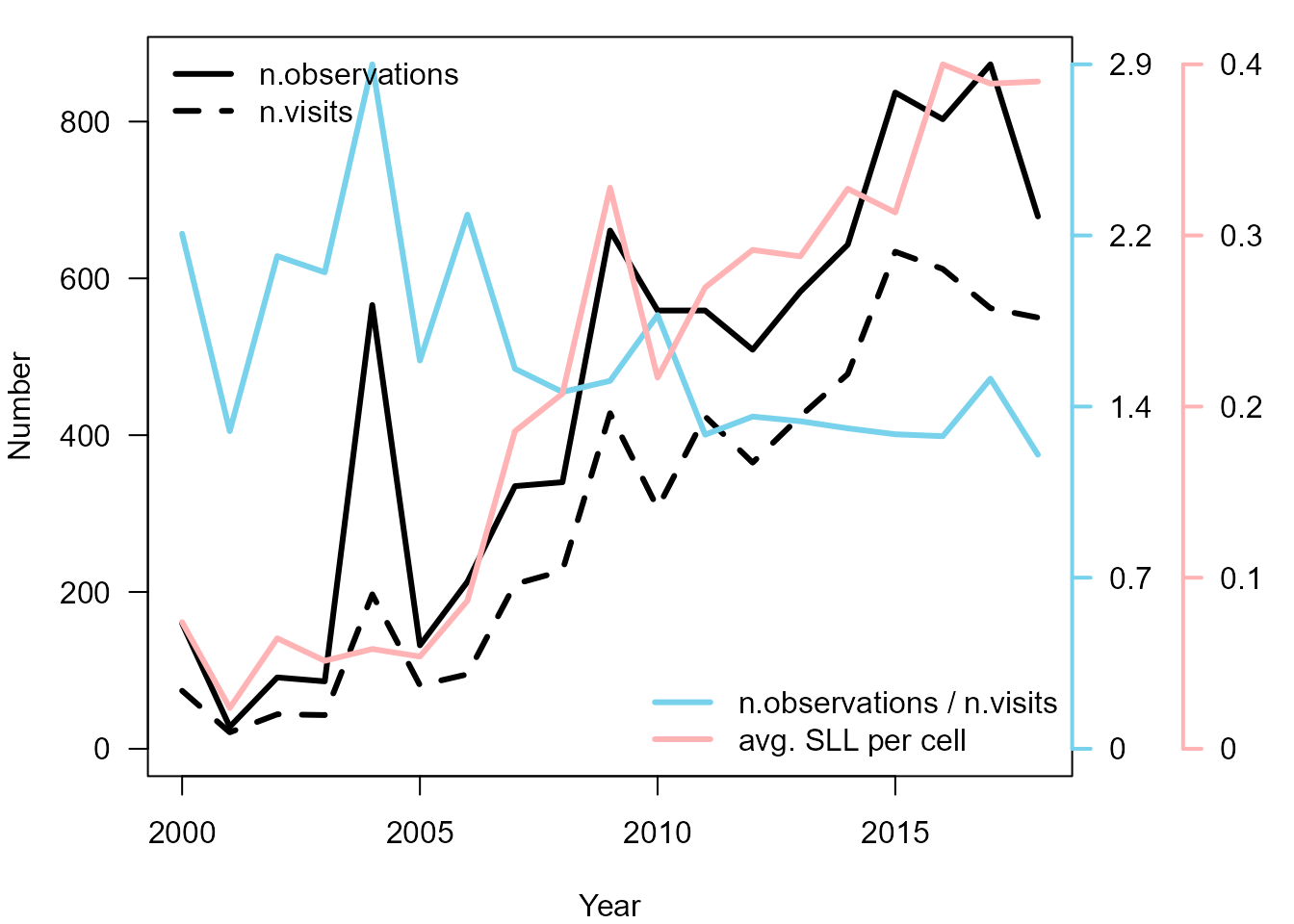
Time series for Bombus spp. dataset.
Although we downloaded the data in April 2019, we know that the latest reports for 2018 were not yet uploaded and we see that in the figure.
We can see that over the years there are on average more observations, more visits and also more species reported for each visit. While it looks like as sampling effort has increased we can also see that there are on average fewer observations per visit. This suggests that the sampling effort per visit has actually decreased. There seem to be many more visits reported in later years driving also an increase in number of observations, but many visits hold only few observations. There seem to be also few visits with long species lists driving the increase of average SLL.
Then, we can summarize spatial data in some maps, to review, for example, Where do we have visits at all?, or How often are visits performed in July vs December?
wNonEmpty <- whichNonEmpty( SB$overlaid )
EB <- exportBirds(SB, "Spatial", "Month", "nYears", "sum")
# because the dimension is "spatial", the result is a 'SpatialPolygonDataFrame'

palBW <- leaflet::colorNumeric(c("white", "navyblue"),
                               c(0, max(st_drop_geometry(EB), na.rm = TRUE)),
                               na.color = "transparent")
oldpar <- par(no.readonly =TRUE)
par(mfrow=c(1,3), mar=c(1,1,1,1))
plot(SB$spatial$geometry[wNonEmpty], col="grey", border = NA)
plot(gotaland$geometry, col=NA, border = "grey", lwd=1, add=TRUE)
mtext("Visited cells", 3, line=-1)

plot(EB$geometry, col=palBW(EB$Jul), border = NA)
plot(gotaland$geometry, col=NA, border = "grey", lwd=1, add=TRUE)
mtext("Number of years for which \nJuly was sampled", 3, line=-2)

plot(EB$geometry, col=palBW(EB$Dec), border = NA)
plot(gotaland$geometry, col=NA, border = "grey", lwd=1, add=TRUE)
mtext("Number of years for which \nDecember was sampled", 3, line=-2)
legend("bottomleft",
       legend=seq(0, max(st_drop_geometry(EB), na.rm = TRUE), length.out = 5),
       col = palBW(seq(0, max(st_drop_geometry(EB), na.rm = TRUE), length.out = 5)),
       title = "Number of years", pch = 15, bty="n")
par(oldpar)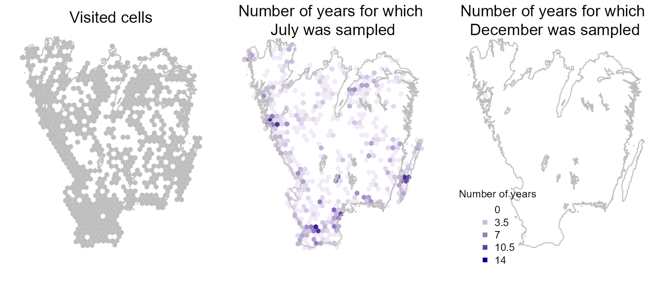
We could also map the ignorance scores based on the either the number of observations or visits using the function exposeIgnorance(). Ignorance scores are a proxy for the lack of sampling effort, computed by making the number of observations relative to a reference number of observations that is considered to be enough to reduce the ignorance score by half (henceforth the Half-ignorance approach). The algorithm behind the Ignorance Score is designed for comparison of bias and gaps in primary biodiversity data across taxonomy, time and space Read more here: Ruete (2015) Biodiv Data J 3:e5361 .
oldpar <- par(no.readonly =TRUE)
par(mfrow=c(1,2), mar=c(1,1,1,1))
palBW <- leaflet::colorNumeric(c("white", "navyblue"),
                               c(0, max(SB$spatial$nVis, na.rm = TRUE)),
                               na.color = "transparent")
seqNVis <- round(seq(0, max(SB$spatial$nVis, na.rm = TRUE), length.out = 5))
plot(SB$spatial$geometry, col=palBW(SB$spatial$nVis), border = NA)
plot(gotaland$geometry, col=NA, border = "grey", lwd=1, add=TRUE)
legend("bottomleft", legend=seqNVis, col = palBW(seqNVis),
      title = "Number of \nobservations", pch = 15, bty="n")

ign <- exposeIgnorance(SB$spatial$nVis, h = 5)
palBWR <- leaflet::colorNumeric(c("navyblue", "white","red"), c(0, 1),
                                na.color = "transparent")
plot(gotaland$geometry, col="grey90", border = "grey90", lwd=1)
plot(SB$spatial$geometry, col=palBWR(ign), border = NA, add=TRUE)
plot(gotaland$geometry, col=NA, border = "grey", lwd=1, add=TRUE)
legend("bottomleft", legend=c(seq(0, 1, length.out = 5), "NA"),
      col = c(palBWR(seq(0, 1, length.out = 5)), "grey90"),
      title = "Ignorance \nnVis, \nO0.5=5", pch = 15, bty="n")
par(oldpar)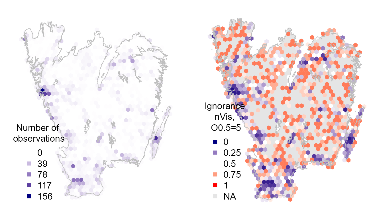
The ignorance scores are highlighting where we have little information and hence cannot be confident about the lack of reports implying an absence of the species.